Recommendations for DC power supplies and USB-based data acquisition hardware for use with ASG's signal conditioners and DC-operated sensors

DC Power Supplies

There are two distinct types of DC power supplies that convert the AC power line voltage into DC voltage to operate electronic devices. Linear supplies use a transformer, rectifier diodes, a regulator, and filtering to produce relatively clean DC, but they are limited to a narrow range of power input voltages and are usually physically large. Switching supplies offer a wider range of power input voltages and are usually smaller in size, but often have switching frequency noise on their DC output. Both types are available in a variety of packages, but most DIN-rail-mounting units are switching supplies.

Because ASG's devices draw relatively low current, the chart of recommended power supplies shown below is based on the number of similar units being powered at the same time. All the power supplies listed below are available from national electronic component distributors such as Digi-Key, Mouser, Newark Electronics, or Allied Electronics at unit prices from $40 to $120. Output Number TDK Lambda Mounting Phoenix Contact Mounting ASG Product

Output Volts DC	Number Devices	TDK Lambda Part Number	Mounting	Phoenix Contact Part Number	Mounting	AFG Product Application
12 V	12	DSP10-12	DIN rail	2868538	DIN rail, tabs	DCSE LVDT
15V	8	DSP10-15	DIN rail			MR, ME, LV LVIT
24 V	6	DSP10-24	DIN rail			LVIT, S2A, SC-200
24 V	10			2868535	DIN rail, tabs	LVIT, S2A, SC-200
24 V	16	DSP30-24	DIN rail	2868648	DIN rail, tabs	LVIT, S2A
24 V	16			2866446	DIN rail only	S2A, SC-200

Data Acquisition Systems

For analog data acquisition (DAQ) input to a PC, the simplest products to utilize are generally USB-based instruments. There are several USB-DAQ choices offered by National Instruments (NI), or their subsidiary, Measurement Computing Corp. (MCC), (which offers more economical DAQ products) that work with ASG products. Typically, USB-based DAQ systems can operate from the 5-Volt DC power of a USB port, so an additional power supply is normally not needed. These DAQ systems work with all the popular NI software like LabVIEW and Signal Express.

DAQ systems are usually used with an analog voltage input, and the majority of ASG products offer a single-ended, ground-referenced DC voltage output up to 10 Volts full scale. Most DAQ systems have at least 8 single-ended analog inputs, and some have differential inputs as well. A DAQ with a differential input capability is of particular benefit for use with sensors that have their DC output off-ground, like some types of DC-LVDTs that offer either a 3-wire connection with a 1-6 Volt grounded output, or a 4-wire hook up with a 0-5 Volt output in which the return side of the output is floating 1 Volt above the ground of the sensor’s power supply.

Recommended USB DAQs for single-ended inputs are the MCC USB200 series and the NI USB-6000 series. Recommended USB DAQs for both single-ended and differential inputs are the MCC USB-1208 series and the NI USB-6008 series. All have a resolution of 12 bits, with a variety of sampling rates available. Detailed product information is available on the respective websites of the suppliers: mccdaq.com or ni.com.

GE Position Sensors on Power Gen Turbines

GE Position Sensors for Power Generation Turbines

How they work and how to operate them with an ASG S2A LVDT signal conditioner

LVDTs (Linear Variable Differential Transformers) are very commonly used as position sensors in power plants throughout the world. Working from AC voltages and frequencies not available from power lines, LVDTs require a signal conditioner to provide the necessary operating power. Alliance Sensors Group's model S2A module, designed specifically to be used in power gen applications, is considered by many power gen users be the most advanced and easy-to-use single channel LVDT signal conditioner on the market today. It can operate practically any LVDT or half-bridge (LVRT) position sensor currently in use.

However, users and systems integrators can be confused by unusual LVDT configurations, particularly in regard to the General Electric 185A1328 and 311A5178 series of LVDTs typically used with their gas turbines. Furthermore, for many years, GE has been using a contactless position sensor known as an inductive half-bridge for measuring the position of the operating shafts of steam turbine control valves. These sensors, often called VRTs or LVRTs, are used to provide position feedback from modulating throttle and governor valves, as well as to give open or closed condition feedback from bypass, stop, and interceptor valves. They are also used to monitor valve position on some turbine feedwater pumps. Some typical GE half-bridge part numbers include the 119C9638, 119C9639, and 196C8768 series. Again, there is some confusion among many systems integrators about how to connect these GE half-bridge sensors to an LVDT signal conditioner and how to calibrate them. This paper should help dispel any confusion about operating an S2A with a GE gas turbine LVDT or steam turbine half-bridge sensor.

Operating GE Gas Turbine LVDTs with an ASG S2A LVDT Signal Conditioner

The first section of this paper shows how these GE LVDTs differ from conventional LVDTs and how to operate them with an S2A LVDT signal conditioner module. To understand the differences between GE Gas Turbine LVDTs and conventional LVDTs, it is important to review the characteristics of an ordinary LVDT. Regardless of the method of construction actually used to make a conventional LVDT, it has a primary winding and two identical secondary windings that are usually connected in series opposition, with a movable permeable core to couple the primary to the secondaries, as shown in Figure 1 below.

The electrical output of a typical LVDT as a function of its core's position is shown in Figure 2 below. Note that the plot of its AC output amplitude versus position shows the classical "V" shape commonly associated with an LVDT, with a minimum value called null at the center of its range of motion, and an increased output amplitude for core positions on either side of null. More important is the fact that the phase relationship of the differential AC output to the primary input voltage shifts abruptly by 180° as the core moves through null. It is this 180° phase shift that permits a user to know on which side of null the core is positioned. The voltages and frequency shown are typical of those found in the operation of a conventional LVDT. It is important to note that the actual excitation voltage utilized makes very little difference to an LVDT's performance. Only the excitation frequency is important for proper operation.

The configuration of the LVDTs used by GE for various position sensing functions on their gas turbines is shown in Figure 3 below. The most obvious difference is the tap on the primary, but otherwise it does not seem to vary much from the view of a conventional LVDT. However, its electrical operation is really substantially different. Although it is tempting to view the primary tap as a center tap, it is not a center tap at all. Most often it is a 30% tap, but on a few models it is a 25% tap. The voltages shown are typical of those used by GE, but, as noted above, the sensor is a differential transformer and will function with whatever AC voltage is applied to operate it. For the sake of clarity, typical GE I/O values are used for the explanation of how this variety of LVDT works.

This LVDT hookup is generally known as a "Buck-Boost" configuration. As can be seen in Figure 3, the voltage at the tap is 30% of the excitation voltage that is being applied to the LVDTs primary, and is in phase with the primary voltage. The way the windings are connected, this 30% voltage, etap, is being added to the differential secondary voltage, which consists of e1, which is in phase with the primary voltage, to which has been added e2, which is 180° out of phase with the primary voltage. The turns ratio of these GE LVDTs is usually about 5:1, so, with a 7.07 V ACrms input, the full scale output of the secondaries, without the effect of the 30% tap, would be about 1.4 V ACrms, either in phase with the primary excitation or 180° out of phase with it. However, the 30% tap inserts an additional 2.1 V ACrms that is in phase with the primary excitation to be added to the voltages already in the secondaries. The result is plotted in Figure 4, which shows that the total AC output from the series connection of the two secondaries and the 30% tap is a voltage between 0.7 to 3.5 V ACrms, with no 180° phase shift as the LVDT's core moves from one end of its range of motion through null to the other end of its range.

The electronics used by GE in their controllers requires this unusual AC output, but almost all these "Buck-Boost" LVDTs can be successfully operated with an ASG S2A signal conditioner module by using the appropriate connection configuration. The first thing to do is to ignore any connection to the primary tap. Instead, connect the LVDT in a 3-wire configuration, as shown in the S2A instruction manual. In this configuration, the high end of the primary is connected to J1-1 (or J1-2, if the output directional sense is reversed), the common connection of the primary and the series-connected secondaries is connected to J1-3, and the secondaries' high output is connected to J1-4. It is also necessary to move jumper J10 to its alternate position and to shift jumper J7 over to its high output position to increase the excitation to the LVDT's primary. After this 3-wire connection for a "Buck-Boost" LVDT has been completed, the S2A can be operated and the LVDT be calibrated in the normal manner shown in the S2A module's manual.

Operating GE Steam Turbine Half-bridge (LVRT) Sensors with an S2A Signal Conditioner

First it is necessary to understand how GE half-bridge sensors function to see how to use them with an S2A signal conditioner. Figure 5 shows the schematic of a typical GE half-bridge sensor. Note that pins D and E play no role in the operation of the sensor, but are merely part of an "interrupt jumper" system which is used to notify the turbine control system that the connector has been removed. As shown in the schematic, the sensor consists of two identically-wound inductor coils connected in series encircling a movable permeable core long enough to overlap a portion of each coil. An AC voltage ein is applied to pins A and C. If the core is located symmetrically between the coils, each coil will have the same impedance and, assuming the output has no load, voltage eout between pins B and C will be 1/2 of ein.

If the core is moved to include more of the coil connected between pins A and B, the inductance, and therefore the impedance, of that winding will increase, while the inductance, and hence the impedance, of the coil connected between pins B and C will decrease. The result will be a drop in the voltage eout. If the core were moved in the other direction, the reverse action would happen and eout would increase.

Thus, the half-bridge acts as an AC voltage divider. Over a limited range of motion, and excited at an appropriate input frequency, this operation can be reasonably linear if the change in impedance of each winding is largely due to its inductance rather than to its DC resistance, as shown in Figure 6 below.

The shaded symmetrical areas represent the different AC output levels developed by different sensors. Several things stand out in Figure 6. First is that the output at mid-range is not zero as with an LVDT, but is half of the AC excitation. Second, there is not a 180° phase shift at "null" as with an LVDT. Both features specifically facilitate interfacing these sensors with GE's Mark 2 - 6 turbine control systems.

There are two other very important points of note in the operation of half-bridge sensors, both of which concern the excitation of the sensors. First, the magnitude of the AC excitation voltage has no bearing at all on the functioning of these sensors. The choice of 7.07 Vrms (20 Vp-p) by GE is merely dependent on the requirements of their control system. Second, the excitation frequency is chosen to make sure the impedance of the two windings is dominated by their inductive reactance at the chosen frequency, so that the DC resistance of the windings has a fairly small overall effect on the winding impedances.

When looking at Figure 6, it is easy to understand why it can be unduly difficult to set up and calibrate these GE half-bridge position sensors in the field. The primary reason is that a half-bridge sensor does not have a uniquely identifiable point in its range of motion like an LVDT's null point. Fortunately, ASG's S2A LVDT signal conditioner was designed not merely to work with inductive half-bridges, but to make their operation emulate that of an LVDT. Thus, anyone familiar with the techniques for calibrating an LVDT position sensor installed in a valve position feedback system using an S2A module will be able to utilize those very same techniques to calibrate a GE half-bridge sensor connected to an S2A module.

Figure 7 below shows that a GE inductive half-bridge connected to an S2A signal conditioner displays exactly the same type of AC output as would be developed if the S2A were connected to an LVDT. When using an S2A with a half-bridge sensor, the front panel LEDs function in the same way during calibration as if it were an LVDT, as does the Null Output voltage available at J4-1 and J4-2. While this app note has focused on the GE half-bridges used in power plants, these same considerations apply to operating any inductive half-bridge sensor with an S2A or any of its derivative LVDT signal conditioners.

The connection diagram for hooking up GE half-bridges to an S2A signal conditioner module is shown above. Hook up the GE half-bridge connector's pins to the numbers on the black plug, J1, as follows: Pin A goes to J1-1, pin B goes to J1-4, and pin C goes to J1-2. Pins E and F are not connected to the S2A at all. Also, move jumpers J7 and J10 over to their alternate positions. If the directional sense of the S2A's analog output is reversed from the desired output, either interchange the connections to J1-1 and J1-2, or flip the INVERT switch, DS2-3, inside of the S2A.

50/60 Hz GE Half-bridge Sensors used with ASG S2A Signal Conditioners in Steam Power Plants

This paper was based on the most common GE half-bridge sensors likely to be found in power plants today, all of which operate at 3 kHz. However, early on, GE used some half-bridge sensors that were operated with 24 Volts AC at 50/60 Hz and some even used 115 Volts AC, 50/60 Hz. Both systems integrators and power gen utilities should be aware of the risks of continuing to use a more than half-century old design of 50/60 Hz-operated GE half-bridges instead of the newer 3 kHz-operated sensors.

These 50/60 Hz units do not contain much ferromagnetic material beyond their core so their windings utilize many turns of fine wire to achieve the needed inductance. As a result, their winding impedance has a large resistive component, so that much of the AC input power gets dissipated in the resistance of the windings, leading these sensors to get quite hot internally during normal operation.

Because of the effects of thermal expansion and contraction on the winding insulation, these 50/60 Hz units have a history of developing intra-winding shorts, but which do not immediately produce significant output changes because there are so many turns of wire on each winding. Furthermore, sensor output linearity is also poor to begin with, typically ± 2% at FSO, and ± 5% at 110% of FSO, which often initially masks the effects of any such internal shorts. But over a period of time, the internal winding shorts can and often do increase, causing a net calibration shift that could result in a significant sensor output error.

Despite these issues, several integrators have had success using these old 50/60 Hz GE half-bridge sensors with an ASG S2A LVDT signal conditioner by operating them with the S2A's 1 kHz excitation frequency. In fact, some old sensors had such a low winding impedance at 1 kHz that it was necessary to operate them at 3 kHz. Typically, those integrators have utilized old stock of unused spares or ordered new units built to the old design, mostly because their utility customers are reluctant to change sensors over to newer, more reliable products, particularly in nuclear power plants, because of issues with certifications, testing, and related documentation. Even so, it is important to bear in mind that these 50/60 Hz sensors utilize a genuinely obsolete design, and that contactless inductive position sensing technology and sensor reliability have improved substantially in the intervening half-century or more.

To download a PDF of this article, please click here.

Specific differences between ASG's S2A and SC-200 LVDT signal conditioner modules

The S2A and SC-200 LVDT signal conditioners are very similar; however, each unit was designed with specific features for the markets it serves in mind, so there are a few differences between them.

The S2A was specifically designed for the power generation industry and has the following features:

LVDT excitation frequencies of 1, 3, 5, and 10kHz. The 1kHz and 3kHz frequencies were selected so the conditioner could be used with GE and Westinghouse steam turbine LVDTs and LVRTs.

If the S2A senses a sensor-related fault, the module's fault-response outputs are activated and in addition, the analog output is driven out of range. This is done so that in a redundant sensor configuration, by using an algorithm coded into the turbine's DCS control system, the faulty reading is identifiable and is not be accepted by the DCS with the other correct sensor readings.

The SC-200 was designed for standard industrial applications and has the following features:

LVDT excitation frequencies of 2.5, 5, 7.5, and 10kHz. The 2.5kHz frequency is commonly used by LVDT manufacturers and the 7.5kHz frequency was selected to be used with Marposs analog pencil gaging probes. Alliance Sensors Group is an official distributor for Marposs USA.

The analog output is NOT driven out of range should the SC-200 sense a fault, but the module's other fault-response outputs are activated.

Click to View Most Commonly Used Signal Conditioners.

How to Use the Failure Warning Output at J2-2 of an ASG LVDT Signal Conditioner

The LVDT signal conditioner module offers an open-collector failure warning output signal which is available at J2-2 on the blue terminal block connector. This output is a connection to the collector of an internal transistor switch, whose factory default mode of operation is Normally Open (NO). In NO mode a device connected between the +24 V DC supply and J2-2 will have no current flow when the module is operating without error, producing a logic High (+24 V) at J2-2, but if a failure occurs, current will flow producing a logic Low (0) at J2-2.

For modules with version 2 firmware, the open-collector switch's mode of operation can be changed in the field from Normally Open (NO) to Normally Closed (NC) by using the SET FOP command over the RS-485 bus. In the NC mode, the device connected between the +24 V DC supply and J2-2 will have current flow if the module is operating without error, producing a logic Low (0) output at J2-2, but if a failure occurs, current flow will stop, producing a logic High (+24) output at J2-2. To determine if this change is possible, find the module's firmware version by using the RS-485 bus command VERSION.

It is important to note that there is a built-in time delay between when a failure is detected and when the transistor actually turns on, which is normally the factory default of 200 ms, but can be reprogrammed in the field from 0 to 900 ms in 100 ms increments using the SET FD command over the RS-485 bus. This time delay prevents "nuisance trips" from unusual transients such as nearby lightning strikes, etc., and applies only to the NO or NC Failure Warning Output at J2-2. It does not affect any other fault indicators built into the S2A like the front-panel LEDs flashing or the analog output being driven out of range.

The types of devices that are typically connected between the +24 V DC supply and the open collector failure warning output terminal J2-2 include:
1. A 10 kilohm "pull-up" resistor for generating a TTL digital logic signal between J2-2 and ground in the event of a failure that can be transmitted to the control room and the DCS or operations data recorder.
2. A magnetic DC relay that requires 50 mA or less to operate, which can operate additional devices such as an audible alarm or an annunciator light. The voltage developed across the relay coil can also be used as in the same way as that across a pull-up resistor to provide a TTL digital logic output signal.
3. A solid-state relay that functions in the same manner as (2) above.
4. An LED array (with appropriate series resistors) for local fault indication.
5. A low wattage 24 Volt incandescent lamp for local fault indication.

Note that the open collector can be used with external devices as long as there is a ground connection from the module in addition to the connection to J2-2, but be careful not to produce a "ground loop".

Hot Swapping S2A LVDT Signal Conditioning Modules

Under the right conditions, an S2A module can be "hot swapped" with another module having the same internal DIP switch settings and loaded with values in certain EEPROM locations that match those in the original module. If S2As are connected in a multi-module array, this process will take the selected module off-line, but if done carefully, will allow the remaining modules in the array to operate normally.

To prepare the replacement module for a hot swap, the configuration data of the original module, which should have been obtained previously and saved for a possible hot swap, is needed. If this data is not available, connect to the RS-485 port of the original module with a PC and terminal program, and use the Config command to get it. Using that data, set the internal DIP switches and jumpers of the new module to match, then power it up and use its RS-485 port as noted above to load the values of ADC HI, ADC Lo, In Pot, Gain, and, if needed, FOP, FD, and LF using the Set command for each value.

To do the hot swap, first disconnect only the input power positive from the original module. Do this by pulling that module’s power input fuse, by tripping its circuit breaker, by turning off its power switch, or by loosening the screw terminal of J4-4, the red plug, and carefully removing the wire connected to it. Do not remove the red plug with any power present. Once the unit has been depowered, the plugs may be removed from the original module in this order: J4 (red), J3 (green), J2 (blue), then J1 (black). Insert the plugs into the replacement module in reverse order: J1 (black), J2 (blue), J3 (green), and last, J4, (red), but with no input power positive. Finally, restore the input power positive or reconnect the wire to J4-4.

Comparison of ASG’s SC-200 to SC-100 LVDT Signal Conditioner Modules

Descriptively, there are several significant improvements of the SC-200 module over its predecessor:

1. The SC-200 now uses plug-in screw terminals, so the I/O connections can be hooked up without being attached to the module.

2. The SC-200 has a fully differential input, which common modes out most ground-loop developed noise signals. The SC-100 has a single-ended input, which is easier to work with, but can be more susceptible to certain types of extraneous noise, usually from shield grounding issues.

3. The SC-200 offers two user-selectable shield grounding points versus the SC-100’s single user-selectable shield grounding point.

4. SC-200 incorporates a user-invoked lockout cybersecurity feature to prevent tampering and to notify a user of a tamper attempt.

5. The SC-200 has improved filtering of the sine wave excitation signal to produce less harmonic distortion than the SC-100’s excitation, which reduces capacitively coupled noise issues arising from long cables.

6. An SC-200 permits changing the module’s excitation frequency and the analog output via ASCII commands over the RS-485 bus, which obviates any need to open the module’s case for this purpose and offers a user complete remote setup for operation with an LVDT. For half-bridge sensors, 2 internal jumpers must be set by the user. An SC-100 does not offer this completely remote setup feature. Note that for either unit, the case must be opened to set the specific digital address.

7. The SC-200 has more system diagnostic capabilities than the SC-100, which can assist in fault detection for high reliability applications. At least 16 fault conditions can be detected by the SC-200’s diagnostics, including shorted, disconnected, or open primary; shorted, grounded, disconnected, or open secondaries; analog voltage output shorts or current loop opens; and the most common hook-up errors made during initial setup and installation.

8. SC-200 has a real-time recalibration feature to tweak the analog output after the mechanical system has warmed up. Recalibration can be performed either over the module’s RS-485 bus or from its front panel.

9. The SC-200 has an SC-100 emulation mode to make it operate essentially the same as an SC-100 for retrofit requirements, although operation as an SC-200 is the preferred mode.

New Features and Diagnostics Comparisons

Features	SC-200	SC-100	Competitor
Differential Input Connection of Sensor’s Output	X		X
Two User-Selectable Shield Grounds	X
Remote Setup of Module via RS-485 bus	X
Remote Calibration via RS-485 bus	X	X	X
Module Hot Swappable	X	X	X
SC-100 Emulation Mode for Backward Compatibility	X
In-Process Recalibration for Zero and/or Full Scale	X	X
Error Output Polarity Configurability as N.O. or N.C.	X	X

Diagnostics
Primary Connection Open	X	X	X
Primary Connection Shorted across leads	X
Primary Connection Shorted to ground	X	X
Secondary Connection Open	X	X	X
Secondary Connection Shorted across Leads	X
Secondary Connection Shorted to ground	X	X
Voltage Output Short	X
Current Loop Output Open	X
Sensor Wiring Errors	X
Shorted Master / Slave Bus	X	X
Module Wiring Errors	X

Cyber Security
Anti-Tampering Lockout	X
Tampering Warning Flag Output	X

Using the RESTORE Function for S2A or SC-200 LVDT Signal Conditioners

An S2A or SC-200 module set for 4-20 mA output displays an output error during setup

1. Before taking any specific remedial action:

a. Make sure that the analog output is not connected into a loop powered system.

b. Make sure that there is a loop load resistor connected to the module's output terminals.

2. If the E and S LEDs are blinking and the P LED is not illuminated, perform the RESTORE function by depressing the front panel ZERO pushbutton 3 time in a row for a least 1/2 second duration each time.

3. If the RESTORE function was successful, the E and S LEDs will go off and the P LED may turn on.

4. If the RESTORE function was unsuccessful, repeat the process, carefully observing the duration.

5. When successful, proceed to calibrating the module with the connected LVDT sensor normally.

Techniques for Measuring the Primary Impedance of an LVDT

Techniques for Measuring the Primary Impedance of an LVDT

Periodically the need arises to be able to measure the primary impedance of an LVDT to ensure that it will work with a particular version of signal conditioning electronics. Typical LVDT signal conditioner systems are built to work with a primary impedance of 200 Ohms or higher, but some systems cannot supply enough excitation power to operate an ordinary industrial LVDT. If a user is uncertain of the primary impedance of a particular LVDT, it may be necessary for that user to actually measure it.

However, before explaining how to do it, it is important to be certain that the user understands that one cannot measure impedance using the resistance ranges of a multimeter, even though they are both measured in Ohms. Those ranges of a multimeter indicate DC resistance (DCR).

Impedance is an AC phenomenon, which is a function of and determined by frequency. There are many inexpensive hand-held instruments that can measure R-L-C circuit element parameters which can then be used to calculate inpedance. However, these devices are often unable to make measurements at the desired frequency. There are also expensive instruments called Impedance Meters that can directly measure the impedance of an R-L-C circuit at some particular frequency. These meters usually have a variable frequency source or some selection of common reference frequencies available to provide an impedance reading. Finally, Impedance Bridges are older laboratory devices to measure impedance by measuring the R-L-C circuit element parameters which can then be used to calculate inpedance

In the absence of direct reading instruments to measure impedance, there is a very fundamental method of measuring the scalar (magnitude) component of the primary impedance of any LVDT on the laboratory bench by using Ohm's Law for AC circuits, as described in the steps below:

1. Make sure the core of the LVDT is approximately at its Null position inside the LVDT's bore.

2. Hook up an audio frequency sine wave oscillator to the LVDT's primary leads or connector, being sure both of the LVDT's secondaries are not connected to anything.

3. Set the oscillator at or near the LVDT's nominal excitation frequency, typically 2.5 or 3.0 kHz.

4. Use a precision true-RMS AC voltmeter with enough bandwidth at the above frequency to measure the voltage being applied to the LVDT's primary at its nominal AC input, typically 3 V.

5. Use a precision true-RMS AC milliameter, again with enough bandwidth at the frequency above, connected in series with the LVDT's primary to measure the AC current being drawn.

6. Use a calculator to divide the RMS voltage from step 4 by the RMS current in step 5. If the AC current is in milliamperes and the AC excitation is in Volts, using Ohm's Law for AC circuits, the quotient is the magnitude in kilohms of the primary impedance at the excitation frequency.

7. To know the LVDT's input power in milliwatts, multiply AC voltage (V) by AC current (mA).

8. For an LVDT that is already connected to an LVDT signal conditioner and being powered at or near the LVDT's nominal excitation frequency, it is only necessary to follow steps 1, 4, 5, and 6 above to gather the parameters needed to calculate the LVDT's primary impedance.

Using the RS-485 Port of ASG S2A/SC-200 LVDT Signal Conditioners

ASG's LVDT signal conditioners incorporate an RS-485 two-wire multi-drop serial communications interface for up to 16 devices. This port enables half-duplex serial communication by which a module can be set up and calibrated remotely and system data can be read or stored on a PC running an ASCII terminal program like Hyper Terminal with a 2-wire RS-485 converter for the computer's com port or USB port connected to terminals J3-1 and J3-2 of the signal conditioner. The PC's com port parameters are: 9600 bps, no parity, 8 data bits, and 1 stop bit (9600, NP, 8, 1), with echo on and no flow control. Be sure that the RS-485 connection for Data A (D-) is connected to J3-2 and Data B (D+) is connected to J3-1. Always follow the data polarity (D) indicated above, regardless of the letters for data lines used by the RS-485 converter.

ASG offers a 1.8 m long 2-wire USB-to-RS-485 converter cable, USB-RS485-WE, p/n 5810-0001, having an orange wire with a red tip plug that is Data B (D+), and a yellow wire and tip plug that is Data A (D-). Normally no driver is needed for a USB-RS485-WE used with MS Windows 7 or later. For Windows XP or earlier, or MAC or Linux operating systems, driver software can be found on: www.ftdichip.com. In most cases, the optimum driver for any particular OS is the VCP version.

RS-485 user commands for S2A/SC-200 ASG LVDT signal conditioner modules

Note that all commands must be formatted to begin with UXX followed by a space, where XX is the numerical value between 00 and 15 of the module's decimal digital address as set up on DS2, switches 5, 6, 7, and 8 according to Table 1b in the S2A instruction manual, or by following the DIP switch settings diagram shown on the S2A module's left side label.

Note: Some Set command descriptions show in bold face the range of values that follow the command and a (space).

Analog In RUN mode, returns the nominal analog output value scaled in electrical units that depend on the setting of DS1, or the analog output range selected with the Set Aout command.

Cal Enters CALIBRATION mode; command is the same as pressing FULL SCALE and ZERO pushbuttons together.

Clrall In RUN mode, clears EEPROM of all RS-485 command settings used to override module's DIP switch settings.

Config Lists the module's setup data and displays DIP switch settings and current EEPROM values. Specifically, it shows the module's firmware version, operating mode, digital address (00 - 15), date stamp, serial number, analog output setting (1 - 8), excitation frequency setting (0 - 3), output invert switch off or on, low frequency filter status (LF) off or on and filter corner frequency, excitation drive jumper (J7) in or out, failure output delay time (FD) and polarity (FOP) NC or NO, Lock status, and stored EEPROM values for ADC Lo, ADC Hi, Input pot, and Gain pot. (Log and store all Config data and values by digital address to be able to reconfigure a hot swapped module at a later time).

Error In RUN mode, displays any setup or operations error code(s); for multiple errors, the error code sum is displayed.

Errsec In RUN mode, ON, OFF (default) toggles error indications and failure outputs from low DCR LVDT secondaries.

Errsig In RUN mode, ON (default), OFF toggles error indications and failure outputs for all errors found during setup.

Exit Required to exit CAL mode, or to exit any Set command writing a value to the module's EEPROM in RUN mode.

FS In CAL mode, sets the module's full scale output point at the LVDT core’s maximum position and is the same as pressing FULL SCALE pushbutton. Occasionally it may require setting a second time after using the Z command.

Help Shows all ASCII user commands available for execution over the RS-485 bus, including a few not shown in this list.

LEDs In RUN and CAL modes, outputs the status of the 3 green LEDs, displayed in S-E-P order, e.g.: - * 0 means S LED is off, E LED is flashing slow, and P LED is on. + is a fast flash and ! indicates alternating solid and flashing.

Lock In RUN mode, locks the module against any changes and displays attempted tampering over the RS-485 bus.

Null In RUN mode, displays the Null Output voltage at any core position and is typically used to verify that the core of an LVDT is at null; may also be used to establish the symmetry of an LVDT’s endpoint outputs versus core position.

Read LF In RUN mode, when DS2-4 is ON, or the LF filter is invoked, shows the status and frequency setting of the supplemental low frequency low pass filter.

Recal FS In RUN mode, after a calibration has been completed, if the actual full scale output value is within ±4% of the nominal full scale output value selected by DS-1 or the Set Aout command, this command trims the actual full scale output value to match the selected full scale output value. The command may be repeated once to get the most precise FS output value. Recal can be set at module by pressing and holding the FULL SCALE button until the POWER LED blinks.

Recal Z In RUN mode, after a calibration has been completed, if the actual zero output value is within ±4% of the nominal zero output value selected by DS-1 or the Set Aout command, this command trims the actual zero output value to match the selected zero output value. This command may be repeated once to get the most precise zero output value. Recal can also be set at the module by pressing and holding the ZERO pushbutton until the POWER LED blinks.

Reset In RUN mode, produces a "soft" reset of the module's processor so the module restarts as if it is powering on. Command is the same as pressing the FULL SCALE pushbutton three times for at least one-half of a second each.

Reset All In RUN mode, using prefix U90 instead of Uxx, this command performs a simultaneous "soft" reset on all modules connected to the RS-485 bus. Each module on the RS-485 bus then restarts itself as if it is powering on.

Restore In RUN mode, resets module to factory set condition by cancelling all user setup values stored in EEPROM. It can also be invoked by pressing the ZERO pushbutton three times in a row for one-half of a second each time.

Set ADC Hi In RUN mode, writes an A/D converter high value into module's EEPROM. Command is used during a hot swap module reconfiguration to enter the ADC Hi value logged from the original module's Config command.

Set ADC Lo In RUN mode, writes an A/D converter low value into module's EEPROM. Command is used during a hot swap module reconfiguration to enter the ADC Lo value logged from the original module's Config command.

Set Aout In RUN mode, permits setting the analog output range: 1 - 8, independent of the setting of DIP switch DS1.

Set Exf In RUN mode, permits setting excitation frequency: 0 - 3, independent of settings of DIP switches DS2-1, -2.

Set FD In RUN mode, permits the user to set the delay time before the failure warning output switch is activated from 0 to 900 msec in 100 msec increments: 0 - 9. The factory default delay time is set at 200 msec.

Set FOP In RUN mode, sets failure warning switch polarity: NC, Normally Closed (default) or NO, Normally Open.

Set Gain In RUN mode, writes a Gain pot value into module's EEPROM. Command is used during a hot swap module reconfiguration to enter the Gain pot value logged from the original module's Config command.

Set In Pot In RUN mode, writes an Input Pot value into module's EEPROM. Command is used during a hot swap module reconfiguration to enter the Input Pot value logged from the original module's Config command.

Set Inv In RUN mode, permits inverting analog output by overriding setting, ON, OFF, of invert DIP switch DS2-3.

Set LF In RUN mode, sets the corner frequency of the supplemental low pass filter between 0.1 Hz and 10 Hz. If DS2-4 is not ON, command permits LF filter status to be changed: ON, OFF, and its corner frequency to be set.

Ver In RUN mode, returns the version number of the module's firmware.

Z In CAL mode, sets the module's zero output point at the minimum position of the LVDT's core; function is the same as pressing the ZERO pushbutton. Occasionally it may require setting a second time after using the FS command.

SC-200 LVDT Signal Conditioner Quick Start Guide

To view the SC-200 Signal Conditioner Start Guide please click here!

S2A LVDT Signal Conditioner Quick Start Guide

To view the S2A Signal Conditioner Start Guide please click here!

4 to 20 mA Current Loops Made Easy

Understanding current loop output sensors

For analog sensor data transmission, a 4-20 mA current loop is a very common method to convey the sensor data acquired. Sensors or transducers are usually designed to measure a range of values of the measured parameter, which is known as the measurand. The measurand value must be converted to current within the measuring device in such a way that the current in the loop will be proportional to the measurand value. The range of the loop current, 4 mA to 20 mA, is called the span of the transmitter. The transmitter is typically configured so that one end point of the measurement value will correspond to 4 mA and the other end point value measured will correspond to 20 mA.

The 4-20 mA current loop has become the standard for signal transmission and electronic control in most analog control systems. A 4-20mA current loop circuit is shown in Figure 1. In a current loop, the current is drawn from a DC loop power supply, then flows through the transmitter using field wiring connected to a loop load resistor in the receiver or controller, and then back to the loop supply, with all elements being connected in a series circuit. All current-loop-based measuring systems use at least these four elements.

Figure 1.Typical 4-20 mA current loop

Advantages of a Current Loop

An obvious question arises: Why use a 4-20 mA current loop to transmit the analog data from a sensor? The answer is that a 4-20 mA current loop offers several benefits for such sensor data transmission:

- A major reason is that the loop current does not vary with long field wiring, as long as the voltage developed in the loop, called the Compliance Voltage, can sustain the maximum loop current.

- Another benefit is that the current loop has a low impedance and is not particularly susceptible to noise or EMI at large.

- A third advantage is the live-zero feature of the loop (the 4 mA low limit), which makes the loop self-diagnostic if there is a break or bad connection in the loop or a loop power supply failure.

- A current loop permits other current operated devices such as a remote readout or a recorder to be put in series with the loop, within the constraints permitted by the loop's Compliance Voltage.

- The low level of maximum loop current (20 mA) allows the use of relatively simple safety barriers to limit loop current to an Intrinsically Safe level that prevents ignition in a Hazardous Location.

Loop Power Supply and Compliance Voltage

When current is transmitted in the loop, there are voltage drops due to the field wiring conductors and any connected devices. However, these voltage drops do not affect the current in the loop as long as the total loop voltage is sufficient to maintain the maximum loop current. The element responsible for maintaining a stable current in the loop (as shown in Figure 1) is the loop DC power supply. The range of voltage over which the loop will function is called its Compliance Voltage. Common values for 4-20 mA loop supplies are 24VDC or 36VDC. The voltage chosen by a designer depends on the number of elements connected in series with the loop, because the loop power supply voltage must always be higher than the sum of all the voltage drops in the circuit, including the field wiring voltage drop. The sum of all these voltage drops is known as the loop's minimum compliance voltage. There are certain requirements that the compliance voltage must be able to fulfill, the two most important of which are:

- The loop power supply voltage must be able to power all the devices in the loop, including the field wiring's voltage drop, when the current is at its maximum value, normally 20 mA.

- The loop power supply maximum voltage output must be equal to or lower than the maximum voltage rating of any device in the loop.

Transmitter

A sensor or transducer that measures a physical parameter, such as temperature, pressure, position, or fluid flow is connected to a signal conditioning circuit that converts the measured parameter value to an electrical output signal such as a voltage or current proportional to the measured physical parameter. If this electrical signal is a 4-20 mA DC output connected into a current loop, the hardware and electronics system which sends this current into the loop is called a transmitter. A transmitter may consist of a single device containing a sensing element and internal electronics, or it may utilize a sensor or transducer connected to separate signal conditioning electronics configured as a 4-20 mA current transmitter.

Field Wiring

The 4-20 mA current circulates in the loop. The distance between the sensor-transmitter combination and the process controller or readout can be several hundreds of feet or more. Field wiring conductors are used in the loop to connect the transmitter to the process monitoring or control hardware. It is important to see them as an element of the loop because they have some resistance and produce a voltage drop, just like any other element in the loop. If the sum of all the voltage drops is higher than the loop power supply compliance voltage, the current will not be proportional to the measured parameter and the system will produce unusable data.

The resistance of the field wiring conductors is normally given in Ohms per length, typically Ohms per 1000 feet, so the total resistance is the product of this value times the length of the wires divided by 1000. Note that the wire length includes the loop conductor going to the receiver and the loop conductor for the current return from the receiver, the sum of which is twice the individual conductor length. The total field wiring resistance is represented by the symbol R_w, as is shown in the diagram. The voltage drop due to the field wiring is given by Ohm’s law as:

Ohm's law equation Where I is in Amperes; R_w is in Ohms; and V_w is in Volts.

Receiver or Process Controller

After the loop current is generated, it must usually be further processed in the system.. For example, the current could be used as feedback to a valve controller to open, close, or modulate the valve in order to initiate or control a process. It is generally easier to perform control functions with a voltage rather than a current. The receiver is the the part of the loop circuit that converts the loop current into a voltage. In Figure 3, the receiver is a simple resistor that is in series with the loop, so from Ohm's Law, the voltage developed across it is directly proportional to the loop current, which is itself proportional to the measured physical parameter, the measurand.

Loop Load Resistor

The load resistor used in a 4-20 mA current loop is not an arbitrary value. For any specified compliance voltage, there is a maximum loop load resistance that will permit full current to be developed in the loop. Exceeding the maximum loop resistance, which must include the resistance of the field wiring, prevents the system from providing the full 20 mA output current in the loop. In the case of a typical current output sensor, whose loop load graph is shown in Figure 2 below, at 18 Volts input, the total loop load can be as high as 550 Ohms. At 24 Volts input, total loop load can be as high as 850 Ohms, and at the system's maximum input of 32 volts, the total loop load can be 1200 Ohms.

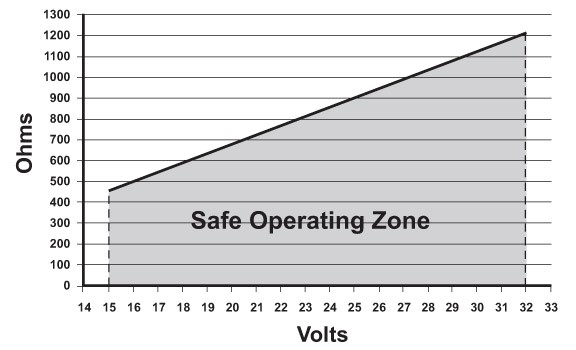
Figure 2 Loop load resistance vs. loop supply voltage for a typical current loop output sensor.

The Importance of Choosing the Right Loop Load Resistor

The choice of the loop load resistor usually depends on the input signal voltage the receiver system requires for good resolution. A 4-20 mA loop current will develop 2-10 VDC across a 500 Ohm load resistor (E = IR). If the receiver system will work satisfactorily with a lower input voltage, the 4-20 mA loop current will develop 1-5 VDC across a 250 Ohm load resistor, which is the most common loop load. Note that a loop load resistor is quite often already built into the receiver input terminal connections. Check the specifications of the receiving device to determine if there is a loop load resistor supplied at its input..

It is very important that the loop load resistor wattage rating is sufficient to ensure that any heating caused by current flowing through the resistor won't change the resistor's value and thereby change the voltage developed across it. Recall that the wattage dissipated by the resistor is I² x R. For a 500 Ohm load resistor, the power dissipated at 20 mA is 0.2 Watts. A good choice for the resistor's power rating is at least 2 Watts because such a load will not heat up very much. Even at full loop current there won’t be a voltage change across the load resistor due to heat from power dissipation instead of actual loop current changes. Note that wire-wound resistors usually have lower temperature coefficients than metallized resistors.

Types of Transmitters

There are several different varieties of current transmitters used for 4-20 mA current loops. In general, they conform to the following categories, delineated by the number of connections required for operation:

- 2-wire transmitters, which usually function as loop-powered current sinking devices.

- 3-wire transmitters, which are independently-powered loop current sourcing devices.

- 4-wire transmitters, which are normally independently-powered devices used when loop isolation is needed for noise or ground loop elimination, or for operation in hazardous locations (hazlocs).

- Derivatives of 4-wire transmitters such as loop isolators or current loop repeaters. Often such devices are incorporated into a national-agency-approved safety barrier for intrinsically safe (IS) systems that can be safely operated in a code-specific hazardous location environment.

2-Wire Current Loop Powered Transmitters

2-wire loop-powered transmitters are electronic devices that can be connected in a current loop without having a separate or independent power source. They are designed to take their power from the current flowing in the loop. Typical loop-powered devices include sensors, transducers, transmitters, repeaters, isolators, meters, recorders, indicators, data loggers, monitors, and many other types of field instruments.

Loop-powered devices are important because for some systems it is difficult to supply separate power to all the devices and instruments in the loop. The device might be located in an enclosure where access might be difficult, or in a hazardous location (hazloc) where power cannot be allowed or must be limited.

Figure 3 shows a 2-wire loop-powered device connected to a current loop. It is considered a current sinking device in the loop circuit. The power to operate the device is supplied entirely by the unused current below 4 mA in the loop. 2-wire loop powered transmitters are popular, but are usually more costly than 3-wire transmitters.

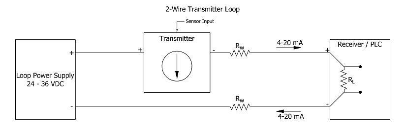
Figure 3 Typical 2-wire loop powered system

3-Wire Current Transmitters

3-wire transmitters are different from loop-powered transmitters because their loop current is developed from a DC power supply that supplies more current than just the loop current. The entire transmitter operates off this supply, and may consume much more current than typical 2-wire loop powered devices. However, a 3-wire system is a sourcing element, so it supplies the current loop despite what it uses itself. 3-wire transmitters are often less costly than 2-wire. A typical 3-wire loop is shown in Figure 4 below. It is important to note that a 3-wire transmitter cannot be connected into a 2-wire loop powered system without significant loop circuit reconfiguration.

Notice the high side of the power supply is not directly connected to the loop, but that the return side of the power supply is connected via a grounded point, so a 3-wire transmitter requires careful consideration of grounding issues to prevent potential ground loops. If an application using a 3-wire transmitter requires isolation in the loop, there are several paths to follow.

One way is to use a separate DC power supply for each 3-wire loop output device, so that there is no interaction with other current loops. Another way is to use a loop isolator module. These devices utilize various methods to achieve galvanic isolation, typically using transformers or optical couplers. They accept a 4-20 mA signal, function as a repeater or re-transmitter, and deliver a reconstituted 4-20 mA current loop signal that is fully isolated. A third way is to use a 4-wire transmitter which has isolation already built in.

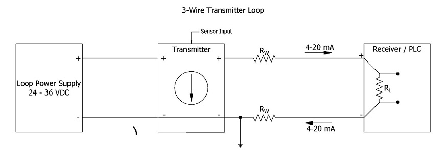
Figure 4 Typical current loop using a 3-wire transmitter

4-Wire Current Transmitters

4-wire transmitters offer the current sourcing advantages of a 3-wire device, but also provide galvanic isolation for the current loop output. 4-wire devices are substantially more expensive than 3-wire devices. For this reason, they are generally used where the isolation is needed, or they are part of a combination device with an approved safety barrier for current loop operation in a specific hazardous location. A 4-wire transmitter block diagram is shown in Figure 5 below. A notable item is that the 4-wire device itself uses a separate DC power supply for operation, just like a 3-wire transmitter, and supplies loop current that way.

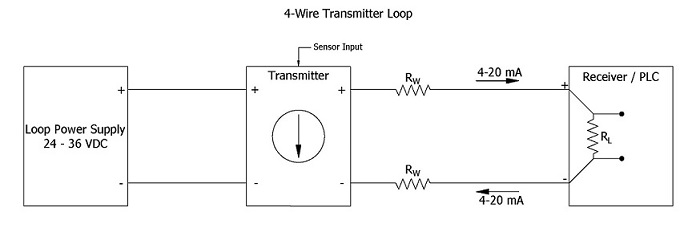
Figure 5 Typical current loop using a 4-wire transmitter

Review of 4-20 mA Data Transmission

The foregoing exposition has provided a brief description of the 4-20 mA current loop data transmission process. It is useful to conclude with a summary of the features and benefits of this process, as well as its limitations.

Advantages

- The 4-20 mA current loop is the dominant data transmission standard in many industries.

- It is recognized as the simplest analog data transmission method to connect and configure.

- It uses less wiring and connections than other methods, greatly reducing startup/setup costs.

- It is superior over long distances of field wiring, as current won't diminish, unlike voltage does.

- It is relatively insensitive to most electrical noise and related EMI (electromagnetic interference).

- It permits a local or a remote readout or monitoring device to be inserted in series with the loop.

- It is self-diagnostic of faults in the measuring system because 4 mA is equal to a 0% system output, so a loop current substantially lower than 4 mA becomes an immediate indicator of a system fault.

Limitations

- 4-20 mA current loops can only transmit one specific sensor or process signal per loop.

- Multiple loops are required for applications where there are many sensor or process outputs that must be transmitted. A lot of field wiring will be needed, which can lead to serious issues with ground loops if the independent current loops are not properly isolated from each other.

- Isolation requirements become exponentially more complicated with a larger number of loops.

LVDT Signal Conditioning Application Notes

DC Power Supplies

Data Acquisition Systems